Transforming Datasets With Pandas

Following from my last blog on Selecting columns and Filtering rows in Pandas, I continue this series on the Python Pandas library for data analysis. Today I wanted to talk about shaping data or transforming data.

Data has a habit of not being ready to use when you receive it. This is why data people tend to spend more then 50% of their time cleaning and shaping data.

I have spoken about tidy data in the past. Tidy data is what data people want to work with but to get the dataset into the shape you want transforming might be needed. Pandas makes it easy by offering some handy dataframe methods.

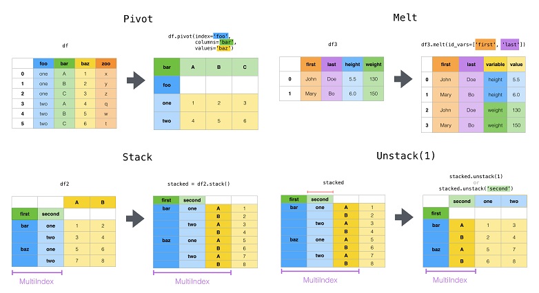
In this post I will look at pivot(), melt(), stack() and unstack()

In [ ]:

import pandas as pd
import numpy as np
import seaborn as sns

Lets load some data from Seaborn https://seaborn.pydata.org/generated/seaborn.load_dataset.html

In [ ]:

# sns.get_dataset_names()
flights = sns.load_dataset('flights')
flights.head()

Out[ ]:

	year	month	passengers
0	1949	Jan	112
1	1949	Feb	118
2	1949	Mar	132
3	1949	Apr	129
4	1949	May	121

Pivot¶

Pivot changes data from tall (tidy) format to wide format, like this:-

In [ ]:

flights = flights.pivot(columns='month', index='year', values='passengers')
flights.head(3)

Out[ ]:

month	Jan	Feb	Mar	Apr	May	Jun	Jul	Aug	Sep	Oct	Nov	Dec
year
1949	112	118	132	129	121	135	148	148	136	119	104	118
1950	115	126	141	135	125	149	170	170	158	133	114	140
1951	145	150	178	163	172	178	199	199	184	162	146	166

To get the dataframe back to were we started we can used stack() with reset_index() which will be discussed shortly.

Melt¶

Melt() allows you to go from wide to tall data. Lets load the flights dateset again.

In [ ]:

flights_wide = pd.read_csv('flights.csv')
print(flights_wide.shape)
flights_wide.head(3)

(12, 13)

Out[ ]:

	year	Jan	Feb	Mar	Apr	May	Jun	Jul	Aug	Sep	Oct	Nov	Dec
0	1949	112	118	132	129	121	135	148	148	136	119	104	118
1	1950	115	126	141	135	125	149	170	170	158	133	114	140
2	1951	145	150	178	163	172	178	199	199	184	162	146	166

Now we melt the dataset from wide to long. It goes from 12 to 144 rows long.

In [ ]:

flights_long = pd.melt(flights_wide, id_vars='year', var_name='month', value_name='passengers_new')
print(flights_long.shape)
flights_long.head(3)

(144, 3)

Out[ ]:

	year	month	passengers_new
0	1949	Jan	112
1	1950	Jan	115
2	1951	Jan	145

To get back to wide data as you know we can just use the pivot method again.

In [ ]:

flights_wide = flights_long.pivot(index='year', columns='month', values='passengers_new')
flights_wide.head(3)

Out[ ]:

month	Apr	Aug	Dec	Feb	Jan	Jul	Jun	Mar	May	Nov	Oct	Sep
year
1949	129	148	118	118	112	148	135	132	121	104	119	136
1950	135	170	140	126	115	170	149	141	125	114	133	158
1951	163	199	166	150	145	199	178	178	172	146	162	184

Stack¶

Stack takes the column index and stacks it in the row index. This lengthens the dataset from 12 to 156 rows.

In [ ]:

print(f'flights_wide shape is: {flights_wide.shape}')
stack_flights = flights_wide.stack()
stack_flights

flights_wide shape is: (12, 12)

Out[ ]:

year  month
1949  Apr      129
      Aug      148
      Dec      118
      Feb      118
      Jan      112
              ... 
1960  Mar      419
      May      472
      Nov      390
      Oct      461
      Sep      508
Length: 144, dtype: int64

As an aside, we can then reset the index to get the data back into columns and rename the values column by chaining dataframe methods.

In [ ]:

flights_wide.stack().reset_index().rename(columns={0:'values'}).head()

Out[ ]:

	year	month	values
0	1949	Apr	129
1	1949	Aug	148
2	1949	Dec	118
3	1949	Feb	118
4	1949	Jan	112

Unstack¶

Unstack does the reverse of stack.

In [ ]:

stack_flights.unstack().head(3)

Out[ ]:

month	Apr	Aug	Dec	Feb	Jan	Jul	Jun	Mar	May	Nov	Oct	Sep
year
1949	129	148	118	118	112	148	135	132	121	104	119	136
1950	135	170	140	126	115	170	149	141	125	114	133	158
1951	163	199	166	150	145	199	178	178	172	146	162	184

Transposing¶

It is quick and easy to transpose your dataset in Pandas, there is even a shortcut!

In [ ]:

flights.head(3)

Out[ ]:

month	Jan	Feb	Mar	Apr	May	Jun	Jul	Aug	Sep	Oct	Nov	Dec
year
1949	112	118	132	129	121	135	148	148	136	119	104	118
1950	115	126	141	135	125	149	170	170	158	133	114	140
1951	145	150	178	163	172	178	199	199	184	162	146	166

In [ ]:

flights.transpose().head(3)

Out[ ]:

year	1949	1950	1951	1952	1953	1954	1955	1956	1957	1958	1959	1960
month
Jan	112	115	145	171	196	204	242	284	315	340	360	417
Feb	118	126	150	180	196	188	233	277	301	318	342	391
Mar	132	141	178	193	236	235	267	317	356	362	406	419

In [ ]:

# Shortcut just use T
flights.T.head(3)

Out[ ]:

year	1949	1950	1951	1952	1953	1954	1955	1956	1957	1958	1959	1960
month
Jan	112	115	145	171	196	204	242	284	315	340	360	417
Feb	118	126	150	180	196	188	233	277	301	318	342	391
Mar	132	141	178	193	236	235	267	317	356	362	406	419

Transformation are an important topic to get your head around, practice will help. That is all for today.

You can read other posts in this series on Pandas via my blog.

---

<

Previous Post

Selecting Columns And Filtering Rows In Pandas

>

Next Post

Grouping Data In Pandas